Quick Start
This short tutorial will demonstrate some of the capabilities of ChiantiPy and the CHIANTI database. It assumes that you know what the CHIANTI database provides and why you want to use it. The current implementation in Version 0.2 mainly provides access to methods concerned with single ions. An ion such as Fe XIV is specified by the string ‘fe_14’, in the usual CHIANTI notation.
Bring up a Python session (using > Python -i ), or better yet, an IPython session
import chianti.core as ch
import numpy as np
import matplotlib.pyplot as plt
What we will really be interested in are various properties of the Fe XIV emissivities as a function of temperature and density. So, let’s define a numpy array of temperatures
t = 10.**(5.8 + 0.05*np.arange(21.))
In ChiantiPy, temperatures are currently given in degrees Kelvin and densities as the number electron density per cubic cm. Then, construct fe14 as would be typically done
fe14 = ch.ion('fe_14', temperature=t, eDensity=1.e+9, em=1.e+27)
note that eDensity is the new keyword for electron density
Level populations
fe14.popPlot()
produces a matplotlib plot window were the population of the top 10 (the default) levels are plotted as a function of temperature.

If the level populations had not already been calculated, popPlot() would have invoked the populate() method which calculates the level populations and stores them in the Population dictionary, with keys = [‘protonDensity’, ‘population’, ‘temperature’, ‘density’].
A ChiantiPy Convention
Classes and function of ChiantiPy start with lower case letters. Data/attributes that are attached to the instantiation of a class will start with a capital letter. For example,
fe14.populate() creates fe14.Population containing the level population information

fe14.emiss() creates fe14.Emiss containing the line emissivity information

fe14.intensity() created fe14.Intensity contain the line intensities information

fe14.spectrum() creates fe14.Spectrum contain the line and continuum spectrum information
Spectral Line Intensities
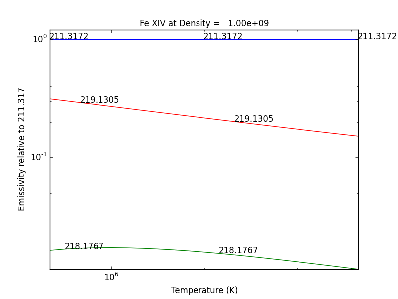
fe14.intensityPlot(wvlRange=[210.,220.],linLog='log')
will plot the intensities for the top (default = 10) lines in the specified wavelength range. If the Intensity attribute has not yet been calculated, it will calculate it. Since there are 21 temperature involved, a single temperature is selected (21/2 = 10). Otherwise,

fe14.intensityPlot(index=2, wvlRange=[210., 220.], linLog = 'log')
plots the intensities for a temperature = t[2] = 7.9e+5, in this case. And, by specifying relative = 1, the emissivities will be plotted relative to the strongest line.

fe14.intensityList(wvlRange=[200,220], index=10)
gives the following terminal output:
 using index =    10 specifying temperature =   2.00e+06, eDensity =    1.00e+09 em =   1.00e+27

 ------------------------------------------

 Ion  lvl1  lvl2                     lower - upper                           Wvl(A)    Intensity      A value Obs
 fe_14     1    11              3s2.3p 2P0.5 - 3s2.3d 2D1.5                  211.3172    2.336e+02     3.81e+10 Y
 fe_14     4    27              3s.3p2 4P1.5 - 3s.3p(3P).3d 4P1.5            212.1255    5.355e-01     2.21e+10 Y
 fe_14     4    28              3s.3p2 4P1.5 - 3s.3p(3P).3d 4D2.5            212.1682    4.039e-01     1.15e+10 Y
 fe_14     3    24              3s.3p2 4P0.5 - 3s.3p(3P).3d 4D0.5            213.1955    8.073e-01     4.26e+10 Y
 fe_14     3    23              3s.3p2 4P0.5 - 3s.3p(3P).3d 4D1.5            213.8822    1.393e+00     2.97e+10 Y
 fe_14     5    28              3s.3p2 4P2.5 - 3s.3p(3P).3d 4D2.5            216.5786    9.736e-01     2.83e+10 Y
 fe_14     5    25              3s.3p2 4P2.5 - 3s.3p(3P).3d 4D3.5            216.9173    1.730e+00     4.29e+10 Y
 fe_14     7    32              3s.3p2 2D2.5 - 3s.3p(3P).3d 2F3.5            218.1767    3.734e+00     1.70e+10 Y
 fe_14     4    22              3s.3p2 4P1.5 - 3s.3p(3P).3d 4P2.5            218.5725    2.391e+00     2.65e+10 Y
 fe_14     2    12              3s2.3p 2P1.5 - 3s2.3d 2D2.5                  219.1305    5.077e+01     4.27e+10 Y

------------------------------------------
optionally, an output file could also be created by setting the keyword outFile to the name of the desired name
fe14.intensityList(wvlRange=[210.,220.], relative=1, index=11)
give the following terminal/notebook output
 using index =    11 specifying temperature =   2.24e+06, eDensity =    1.00e+09 em =   1.00e+27

 ------------------------------------------

 Ion  lvl1  lvl2                     lower - upper                           Wvl(A)    Intensity      A value Obs
 fe_14     1    11              3s2.3p 2P0.5 - 3s2.3d 2D1.5                  211.3172    1.000e+00     3.81e+10 Y
 fe_14     4    27              3s.3p2 4P1.5 - 3s.3p(3P).3d 4P1.5            212.1255    2.267e-03     2.21e+10 Y
 fe_14     4    28              3s.3p2 4P1.5 - 3s.3p(3P).3d 4D2.5            212.1682    1.694e-03     1.15e+10 Y
 fe_14     3    24              3s.3p2 4P0.5 - 3s.3p(3P).3d 4D0.5            213.1955    3.390e-03     4.26e+10 Y
 fe_14     3    23              3s.3p2 4P0.5 - 3s.3p(3P).3d 4D1.5            213.8822    5.891e-03     2.97e+10 Y
 fe_14     5    28              3s.3p2 4P2.5 - 3s.3p(3P).3d 4D2.5            216.5786    4.083e-03     2.83e+10 Y
 fe_14     5    25              3s.3p2 4P2.5 - 3s.3p(3P).3d 4D3.5            216.9173    7.085e-03     4.29e+10 Y
 fe_14     7    32              3s.3p2 2D2.5 - 3s.3p(3P).3d 2F3.5            218.1767    1.557e-02     1.70e+10 Y
 fe_14     4    22              3s.3p2 4P1.5 - 3s.3p(3P).3d 4P2.5            218.5725    1.009e-02     2.65e+10 Y
 fe_14     2    12              3s2.3p 2P1.5 - 3s2.3d 2D2.5                  219.1305    2.096e-01     4.27e+10 Y

------------------------------------------
G(n,T) function
fe14.gofnt(wvlRange=[210., 220.],top=3)
brings up a matplotlib plot window which shows the emissivities of the top (strongest) 3 lines in the wavelength region from 210 to 220 Angstroms.
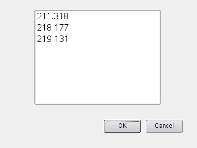
quickly followed by a dialog where the line(s) of interest can be specified
and finally a plot of the G(n,T) function for the specified lines(s).
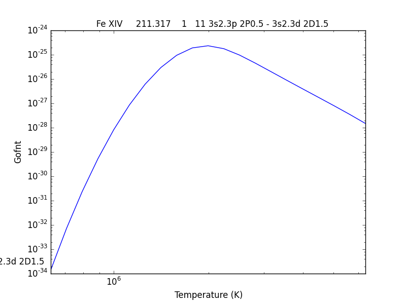
The G(n,T) calculation is stored in the Gofnt dictionary, with keys = [‘gofnt’, ‘temperature’, ‘density’]
while the is a fairly straightforward way to get a G(T) function, it is not very practical to use for a more than a handful of lines. For if the fe_14 line at 211.3172 is in a list of lines to be analyzed, a more practical way is the following
fe14.intensity()
dist = np.abs(np.asarray(fe14.Intensity['wvl']) - 211.3172)
idx = np.argmin(dist)
print(' wvl = %10.3f '%(fe14.Intensity['wvl'][idx]))
prints
wvl = 211.317
plt.loglog(temp,fe14.Intensity['intensity'][:,idx])
once the axes are properly scaled, this produces the same values as fe14.Gofnt[‘gofnt’]

Intensity Ratios
fe14.intensityRatio(wvlRange=[210., 225.])
this brings up a plot showing the relative emissivities on the Fe XIV lines
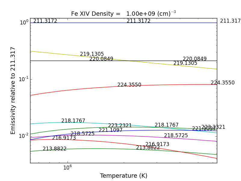
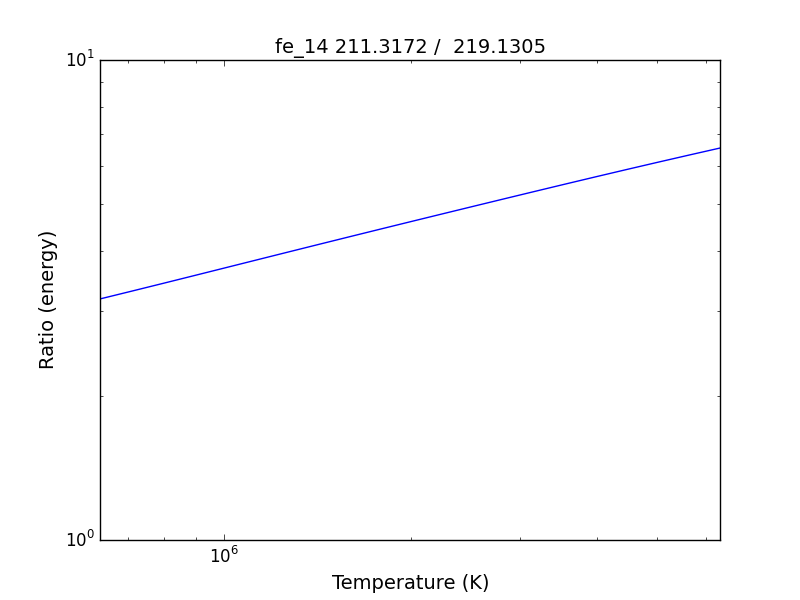
following by a dialog where you can selector the numerator(s) and denominator(s) of the desired intensity ratio
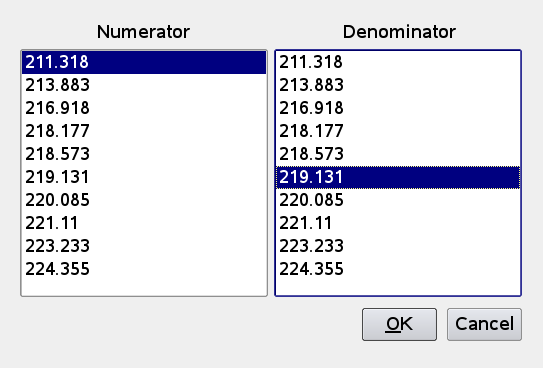
so the specified ratio is then plotted
if previously, we had done
dens = 10.**(6. + 0.1*arange(61))
fe14 = ch.ion('fe_14', 2.e+6, dens)
fe14.intensityRatio(wvlRange=[210., 225.])
then the plot of relative intensities vs density would appear
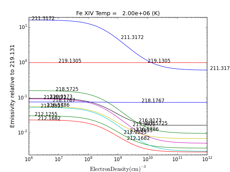
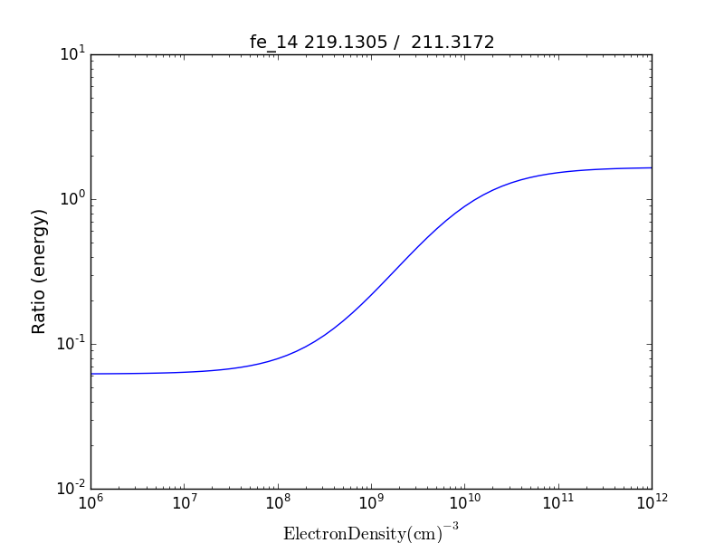
the same numerator/denominator selector dialog would come up and when 2 or more lines are selected, the intensity ratio versus density appears.
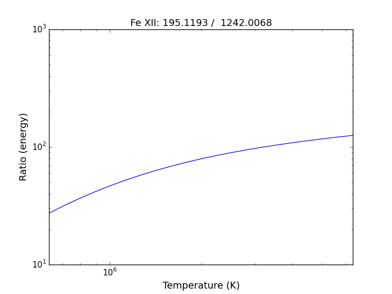
to obtain ratios of lines widely separated in wavelength, the wvlRanges keyword can be used:
fe12 = ch.ion('fe_12', temperature=t, eDensity=1.e+9
fe12.intensityRatio(wvlRanges=[[190.,200.],[1240.,1250.]])
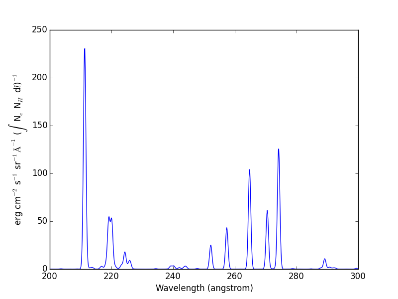
Spectra of a single ion
fe14 = ch.ion('fe_14', temperature = 2.e+6, density = 1.e+9)
wvl = wvl=200. + 0.125*arange(801)
fe14.spectrum(wvl, em=1.e+27)
plot(wvl, fe14.Spectrum['intensity'])
this will calculate the spectrum of fe_14 over the specified wavelength range and filter it with the default filter which is a gaussian (filters.gaussianR) with a ‘resolving power’ of 1000 which gives a gaussian width of wvl/1000.

other filters available in chianti.filters include a boxcar filter and a gaussian filter where the width can be specified directly
if hasattr(fe14,'Em'):
    print(' Emission Measure = %12.2e'%(fe14.Em))
else:
    print(' the value for the emission measure is unspecified')
Emission Measure = 1.00e+27
import chianti.filters as chfilters
fe14.spectrum(wvl,filter=(chfilters.gaussian,.04))
calculates the spectrum of fe_14 for a gaussian filter with a width of 0.04 Angstroms. The current value of the spectrum is kept in fe14.Spectrum with the following keys:
for akey in sorted(fe14.Spectrum.keys()):
    print(' %10s'%(akey))
allLines em filter filterWidth intensity wvl xlabel ylabel
plot(wvl,fe14.Spectrum['intensity'])
plt.xlabel(fe14.Spectrum['xlabel'])
plt.ylabel(fe14.Spectrum['ylabel'])
New in ChiantiPy 0.6, the label keyword has been added to the ion.spectrum method, and also to the other various spectral classes. This allows several spectral calculations for different filters to be saved and compared
temp = 10.**(5.8 + 0.1*np.arange(11.))
dens = 1.e+9
fe14 = ch.ion('fe_14', temp, dens)
emeas = np.ones(11,'float64')*1.e+27
wvl = 200. + 0.125*np.arange(801)
fe14.spectrum(wvl,filter=(chfilters.gaussian,.4),label='.4',em=emeas, label='0.4')
fe14.spectrum(wvl,filter=(chfilters.gaussian,1.),label='1.', label-'1.0')
plt.plot(wvl,fe14.Spectrum['.4']['intensity'][5])
plt.plot(wvl,fe14.Spectrum['1.']['intensity'][5],'-r')
plt.xlabel(fe14.Spectrum['.4']['xlabel'])
plt.ylabel(fe14.Spectrum['.4']['ylabel'])
plt.legen(loc='upper right')

Free-free and free-bound continuum
The module continuum provides the ability to calculate the free-free and free-bound spectrum for a large number of individual ions. The two-photon continuum is produced only by the hydrogen-like and helium-like ions
temperature = 2.e+7
c = ch.continuum('fe_25', temperature = temperature)
wvl = 1. + 0.002*arange(4501)
c.freeFree(wvl)
plot(wvl, c.FreeFree['rate'])
c.freeBound(wvl)
plot(wvl, c.FreeBound['rate'])
fe25=ch.ion('fe_25',2.e+7,1.e+9,em=1.e+27)
fe25.twoPhoton(wvl)
plt.plot(wvl,fe25.TwoPhoton['rate'],label='2 photon')
plt.legend(loc='upper right')
produces

In the continuum calculations, the specified ion, Fe XXV in this case, is the target ion for the free-free calculation. For the free-bound calculation, specified ion is also the target ion. In this case, the radiative recombination spectrum of Fe XXV recombining to form Fe XXIV is returned.
The multi-ion class Bunch
The multi-ion class bunch [new in v0.6] inherits a number of the same methods inherited by the ion class, for example intensityList, intensityRatio, and intensityRatioSave. As a short demonstration of its usefulness, Widing and Feldman (1989, ApJ, 344, 1046) used line ratios of Mg VI and Ne VI as diagnostics of elemental abundance variations in the solar atmosphere. For that to be accurate, it is necessary that the lines of the two ions have the same temperature response.
t = 10.**(5.0+0.1*np.arange(11))
bnch=ch.bunch(t,1.e+9,wvlRange=[300.,500.],ionList=['ne_6','mg_6'],abundanceName='unity')
bnch.intensityRatio(wvlRange=[395.,405.],top=7)
produces and initial plot of the selected lines, a selection widget and finally a plot of the ratio


there seems to be a significant temperature dependence to the ratio, even though both are formed near 4.e+5 K.
A new keyword argument keepIons has been added in v0.6 to the bunch and the 3 spectrum classes.
dwvl = 0.01
nwvl = (406.-394.)/dwvl
wvl = 394. + dwvl*np.arange(nwvl+1)
bnch2=ch.bunch(t, 1.e+9, wvlRange=[wvl.min(),wvl.max()], elementList=['ne','mg'], keepIons=1,em=1.e+27)
bnch2.convolve(wvl,filter=(chfilters.gaussian,5.*dwvl))
plt.plot(wvl, bnch2.Spectrum['intensity'][6],label='Total')
plt.title('Temperature = %10.2e for t[6]'%(t[6]))
elapsed seconds = 11.000 elapsed seconds = 0.000e+00
for one in sorted(bnch2.IonInstances.keys()):
  print('%s'%(one))
yields:
mg_10 mg_10d mg_3 mg_4 mg_5 mg_6 mg_8 mg_9 ne_10 ne_2 ne_3 ne_5 ne_6 ne_8
these IonInstances have all the properties of the Ion class for each of these ions
plt.plot(wvl,bnch2.IonInstances['mg_6'].Spectrum['intensity'][6],'r',label='mg_6')
plt.legend(loc='upper left')
produces

Spectra of multiple ions and continuum
the spectrum for all ions in the CHIANTI database can also be calculated
The spectrum for a selection of all of the ions in the CHIANTI database can also be calculated. There are 3 spectral classes.
- spectrum - the single processor implementation that can be used anywhere
- mspectrum - uses the Python multiprocessing class and cannot be used in a IPython qtconsole or notebook
- ipymspectrum [new in v0.6] - uses the IPython parallel class and can be used in a IPython qtconsole or notebook
The single processor spectrum class
temperature = [1.e+6, 2.e+6]
density = 1.e+9
wvl = 200. + 0.05*arange(2001)
emeasure = [1.e+27 ,1.e+27]
s = ch.spectrum(temperature, density, wvl, filter = (chfilters.gaussian,.2), em = emeasure, doContinuum=0, minAbund=1.e-5)
subplot(311)
plot(wvl, s.Spectrum['integrated'])
subplot(312)
plot(wvl, s.Spectrum['intensity'][0])
subplot(313)
plot(wvl, s.Spectrum['intensity'][1])
produces

The integrated spectrum is formed by summing the spectra for all temperatures.
- For minAbund=1.e-6, the calculatation takes 209 s on a 3.5 GHz processor.
- For minAbund=1.e-5, the calculatation takes 122 s on a 3.5 GHz processor.
The filter is not applied to the continuum.
Calculations with the Spectrum module can be time consuming. One way to control the length of time the calculations take is to limit the number of ions with the ionList keyword and to avoid the continuum calculations by setting the doContinuum keyword to 0 or False. Another way to control the length of time the calculations take is with the minAbund keyword. It sets the minimum elemental abundance that an element can have for its spectra to be calculated. The default value is set include all elements. Some usefull values of minAbund are:
- minAbund = 1.e-4, will include H, He, C, O, Ne
- minAbund = 2.e-5 adds N, Mg, Si, S, Fe
- minAbund = 1.e-6 adds Na, Al, Ar, Ca, Ni
The multiple processor mspectrum class
Another way to speed up calculations is to use the mspectrum class which uses multiple cores on your local computer. It requires the Python multiprocessing module which is available with Python versions 2.6 and later. mspectrum is called in the same way as spectrum but you can specify the number of cores with the proc keyword. The default is 3 but it will not use more cores than are available on your machine. For example,
s = ch.mspectrum(temperature, density ,wvl, em=emeasure, filter = (chfilters.gaussian,.005), proc=4)
The multiple processor ipymspectrum class
next, we will use the ipymspectrum class. First, it is necessary to start up the cluster. In some shell
> ipcluster start –n=4
or, if you are using Python3
> ipcluster3 start –n=4
this will start 4 engines if you have 4 cores but it won’t start more than you have
then in an IPython notebook or qtconsole
temp = [1.e+6, 2.e+6]
dens = 1.e+9
wvl = 200. + 0.05*np.arange(2001)
emeasure = [1.e+27 ,1.e+27]
s = ch.ipymspectrum(temp, dens, wvl, filter = (chfilters.gaussian,.2), em = emeasure, doContinuum=1, minAbund=1.e-5, verbose=0)
plt.figure
plt.plot(wvl, s.Spectrum['integrated'])
produces

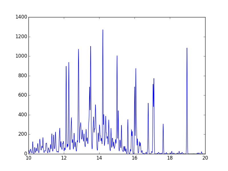
spectrum, mspectrum and ipymspectrum can all be instantiated with the same arguments and keyword arguments. Most of the examples below use the ipymspectrum class for speed.
temperature = 1.e+7
wvl = 10. + 0.005*arange(2001)
s = ch.ipymspectrum(temperature, density, wvl, filter = (chfilters.gaussian,.015))
plot(wvl, s.Spectrum['intensity'])
produces
It is also possible to specify a selection of ions by means of the ionList keyword, for example, ionList=[‘fe_11’,’fe_12’,’fe_13’]
s2 = ch.ipymspectrum(temp, dens, wvl, filter = (chfilters.gaussian,.2), em = emeasure, doContinuum=0, keepIons=1, elementList=['si'], minAbund=1.e-4)
plt.subplot(211)
plt.plot(wvl,s2.Spectrum['intensity'][0])
plt.ylabel(r'erg cm$^{-2}$ s$^{-1}$ sr$^{-1} \AA^{-1}$')
plt.subplot(212)
plt.plot(wvl,s2.IonInstances['si_9'].Spectrum['intensity'][0])
plt.ylabel(r'erg cm$^{-2}$ s$^{-1}$ sr$^{-1} \AA^{-1}$')
plt.xlabel(r'Wavelength ($\AA$)')
plt.title('Si IX')

Because keepIons has been set, the ion instances of all of the ions are maintained in the s2.IonInstances dictionary. It has been possible to compare the spectrum of all of the ions with the spectrum of a single ion.
temp=2.e+7
dens=1.e+9
wvl = 1. + 0.002*np.arange(4501)
s3 = ch.ipymspectrum(temp, dens, wvl, filter = (chfilters.gaussian,.015),doContinuum=1, em=1.e+27,minAbund=1.e-5,verbose=0)
plt.plot(wvl, s3.Spectrum['intensity'])

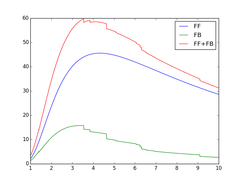
with doContinuum=1, the continuum can be plotted separately
plot(wvl, s3.Spectrum['intensity'])  plot(wvl,s.FreeFree['intensity'])
plot(wvl,s.FreeBound['intensity'])
plot(wvl,s.FreeBound['intensity']+s.FreeFree['intensity'])
produces
temperature = 2.e+7
density = 1.e+9
em-1.e+27
wvl = 1.84 + 0.0001*arange(601)
s4 = ch.ipymspectrum(temperature, density ,wvl, filter = (chfilters.gaussian,.0003), doContinuum=1, minAbund=1.e-5, em=em, verbose=0)
produces

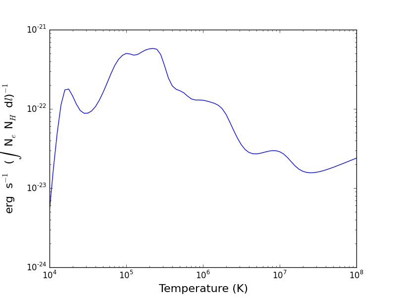
Radiative loss rate
the radiative loss rate can be calculated as a function of temperature and density:
temp = 10.**(4.+0.05*arange(81))
rl = ch.radLoss(temp, 1.e+4, minAbund=2.e-5)
rl.radLossPlot()
produces, in 446 s:
the radiative losses are kept in the rl.RadLoss dictionary
the abundancdName keyword argument can be set to the name of an available abundance file in XUVTOP/abund
if abundanceName=1, a dialog will come up so that a abundance file can be selected